training a model for Washington DC bikeshare kaggle competition with Python

Train a model to predict bike rental volumes using scikit-learn model.
Using the features engineered in my previous blog, we will train a model to predict casual and registered bike volumes.

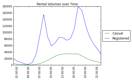
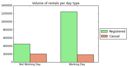
I chose to seperate these two predictions because they have different volume trends. See the two graphs below that show how casual and registered volume trends differ compared for time of day, and whether it is a working day.

Model for casual counts

First we split the feature vector X_vec and target vector Y_vec_cas into training and cross validation sets.

# split into train and cross validation sets for all features
X_train, X_cv, Y_train, Y_cv = train_test_split(X_vec, Y_vec_cas, test_size=0.2, random_state=42)

Train a linear model

Using the sci-kit learn cheat sheet helps us to decide which models to start with.

We are predicting a quantity using a training set of less than 100K samples and all of the features may be important. So we should start looking at models for data with a linear relationship. In the following code, a Ridge Regression model is trained using the training data, and then the R^2 score is calculated using the cross validation data. The R^2 score is only 46%, so it looks like the relationships are not linear.

clf = Ridge(alpha=1.0)
clf.fit(X_train,Y_train)
clf.score(X_cv, Y_cv)

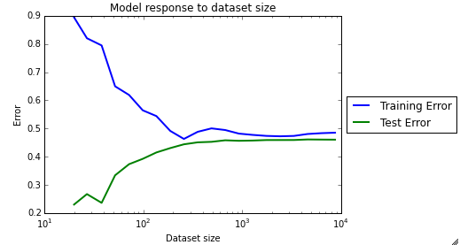
If we take a look at the learning curve, we can see that the training and test error are very similar, which indicates high bias. This confirms that the model is not a good fit at all.

Train an SVR model

To model non-linear relationships, the Support Vector Regression (SVR) model using an rbf kernel can be very effective. We will need to tune the parameters gamma and C using a grid search. This gets an R^2 score of 88% which is a big improvement.

tuned_parameters = [{'kernel': ['rbf'], 'gamma': [1, 1e-1, 1e-2],
                     'C': [100, 1000, 10000]}]

clf = GridSearchCV(svm.SVR(), tuned_parameters, scoring='r2', n_jobs=-1)
clf.fit(X_train,Y_train)

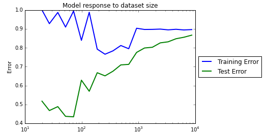
The learning curve for this model looks much more healthy.

Train an ensemble regressor

Since we know we are in the right ball park model, let’s try a Random Forest Regressor. The larger the number of decision trees built, n_estimators, the more accurate the model will be. I’m just using my laptop, so will stick with 1000 for now. This gets an R^2 score of 92% which is pretty good!

clf = RandomForestRegressor(n_estimators=1000)
clf.fit(X_train,Y_train)
clf.score(X_cv, Y_cv)

Model for registered counts

If we run through the same steps as above for casual counts, we find our best model for registered counts is also a Random Forest Regressor with an R^2 score of 95%. I’ve included the code that gets us to this optimal model.

X_train, X_cv, Y_train, Y_cv = train_test_split(X_vec, Y_vec_reg, test_size=0.2, random_state=42)
clf2 = RandomForestRegressor(n_estimators=1000)
clf2.fit(X_train,Y_train)

Predict volumes for test data

The test set features must be engineered, vectorized, standaridized and encoded in the same way as the training features were in my previous blog. Then we predict casual and registered volumes, and the total is our final prediction.

casPredict = clf.predict(X_vec_test)
regPredict = clf2.predict(X_vec_test)

casPredict[casPredict<0]=0
regPredict[regPredict<0]=0

totPredict = casPredict + regPredict

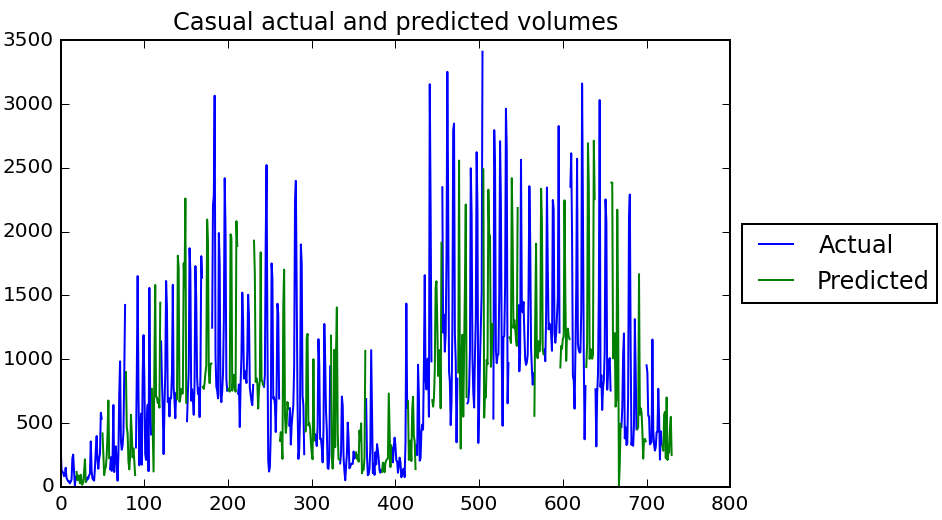
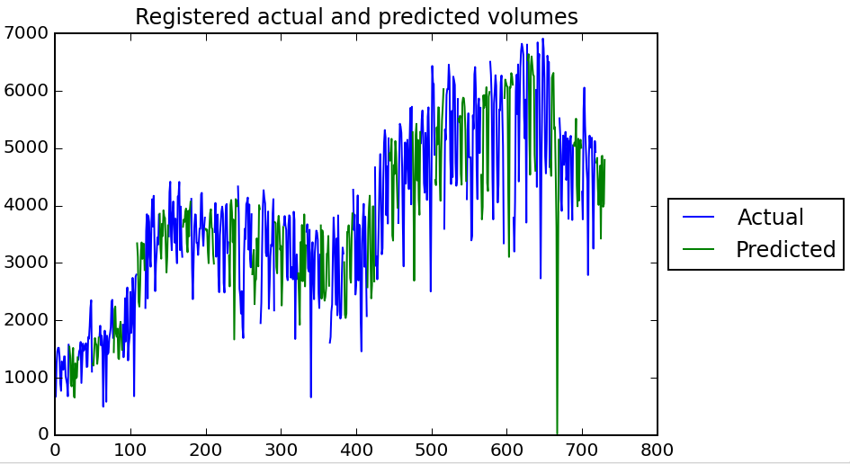
A plot of the actual and predicted volumes over time shows that the model looks pretty logical :)

Feedback

Always feel free to get in touch with other solutions, general thoughts or questions.